- April 5, 2019
- Posted by: Sujithra S
- Category: Data & Analytics

Introduction
Statistics is a solid tool for performing the art of Data Science. Generally anyone can say that statistics is a mathematical body that pertains collecting, analyzing, interpreting and drawing conclusions from the gained information.
With statistics we get to work with data in more informative and targeted way than obtaining from the basic visualization charts.
The math involved statistics helps us to tackle conclusions about our data rather than just estimating.
Statistics in short is study about the data were we can get deeper knowledge and find more insights and also how the data is been structured .
Statistics mainly involves differential statistics (It is a summary statistic that quantitatively describes or summarizes features of a collected Information) and inferential statistics (techniques used to obtain probability making decisions and to find accurate predictions)
Statistical Quantities
The five basic statistical qualities mainly involve Mean, Median, Mode, Variance and standard deviation.
Mean, Median, Mode are also called Central Tendency. Central tendency (or measure of central tendency) is a central or typical value for a probability distribution.
It may also be called a center or location of the distribution.
A central tendency can be calculated for either a finite set of values or for a theoretical distribution, such as the normal distribution.

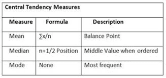
Mean: Arithmetic mean (or simply, mean) is the sum of all measurements divided by the number of observations in the data set
Median: The middle value that separates the higher half from the lower half of the data set. The median and the mode are the only measures of central tendency that can be used for ordinal data, in which values are ranked relative to each other but are not measured absolutely as it is also known as 50th percentile
Mode: The mode of a set of data values is the value that appears most often. It is the value x at which its probability mass function takes its maximum value.
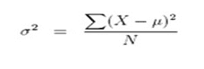
Variance: It measures how far a set of numbers are spread out from their mean. It is calculated by taking the differences between each number in the set and the mean, squaring the differences and dividing the sum of the squares by the number of values in the set.

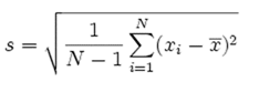
Standard Deviation: It tells you how much data deviates from the actual mean. It is the square root of the Variance.
A low standard deviation indicates that the data points tend to be close to the mean, while a high standard deviation indicates that the data points are spread out over a wider range of values.
A useful property of the standard deviation is that, unlike the variance, it is expressed in the same units as the data.

Discrete Vs Continuous
Discrete variables are countable in a finite amount of time. For Example, the total number of students in the class, or the amount you deposited in the bank account as they all are still countable
Continuous data technically have an infinite number of steps. For Example, A person’s height could be any value (within the range of human heights), not just certain fixed heights.
Distributions
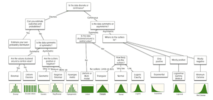
Fitting the Right Distribution
When confirmed with what data needs to be characterized by the distributed, it is always best to start with the raw data trying to fit the right distribution to that data.
As it mainly satisfies basic questions that can help in the characterization. The first is checks the data to the either discrete or continuous.
The second looks for the symmetry and if there is any asymmetry in other words the positive or negative outliers are equal or likely more than the other.
The third relates to the upper and lower limits of data relates to the likelihood of observing extreme values in the distribution; in some data, the extreme values occur very infrequently whereas in others, they occur more often.

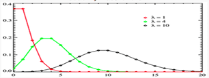
The Poisson Distribution
History: Poisson Distribution was named after French mathematician Siméon Denis Poisson
Description: The Poisson distribution is used to calculate the number of events that might occur in a continuous time interval.
The Poisson distribution can also be used for the number of events in other specified intervals such as distance, area or volume.
For instance, how many Emails might occur at any time where the key parameter that is required is the average number of events in the given interval.
The resulting distribution looks like the binomial, with the skewness being positive but decreasing with l.


Probability of events for a Poisson distribution:
Where,
l lambda is the average number of events per interval
E is the number 2.71828.
k takes values 0, 1, 2, …
k! k × (k − 1) × (k − 2) × … × 2 × 1 is the factorial of k.
This equation is the probability mass function (PMF) for a Poisson distribution
Poisson Distribution Example
The average number of homes sold by the Acme Realty company is 2 homes per day. What will be the probability that exactly 3 homes will be sold tomorrow?
This is a Poisson experiment in which we know the following:
μ = 2; since 2 homes are sold per day, on average.
x = 3; since we want to find the likelihood that 3 homes will be sold tomorrow.
e = 2.71828; since e is a constant equal to approximately 2.71828.
formula:
P(x; μ) = (e-μ) (μx) / x!
P(3; 2) = (2.71828-2) (23) / 3!
P(3; 2) = (0.13534) (8) / 6
P(3; 2) = 0.180
Thus, the probability of selling 3 homes tomorrow is 0.180 .
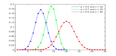
Binomial Distribution
History: Swiss mathematician Jakob Bernoulli, determined the probability of k such outcomes.
Description: The binomial distribution measures the probabilities of the number of successes over a given number of trials with a specified probability of success in each try it is a statistical experiment with consists n repeated trials.
Each trial can result in just two possible outcomes known as success and the other, a failure.
The probability of success, denoted by P, is the same on every trial. A single success/failure experiment is also called a Bernoulli trial or Bernoulli experiment and a sequence of outcomes is called a Bernoulli process; for a single trial, i.e., n = 1, the binomial distribution is a Bernoulli distribution.
The binomial distribution is the basis for the popular binomial test of statistical significance.

Binomial Formula
Suppose a binomial experiment consists of n trials and results in x successes. If the probability of success on an individual trial is P, then the binomial probability is:
b(x; n, P) = nCx * Px * (1 – P)n – x
or
b(x; n, P) = { n! / [ x! (n – x)! ] } * Px * (1 – P)n – x
where,
x Number of successes that result from the binomial experiment.
N Number of trials in the binomial experiment
P Probability of success on an individual trial
Q Probability of failure on an individual trial equal to 1 – P
n! The factorial of n
b(x; n, P) Binomial probability
nCr Number of combinations
Binomial Distribution Example:
Suppose a die is tossed 5 times. What is the probability of getting exactly 2 fours?
This is a binomial experiment in which the number of trials is equal to 5, the number of successes is equal to 2, and the probability of success on a single trial is 1/6 or about 0.167. Therefore, the binomial probability is:
b(2; 5, 0.167) = 5C2 * (0.167)2 * (0.833)3
b(2; 5, 0.167) = 0.161
Negative Binomial Distribution: Assume that the number of successes is fixed at a given number and estimate the number of tries is obtained before reaching the specified number of successes.
The resulting distribution is called the negative binomial and it very closely resembles the Poisson.
In fact, the negative binomial distribution converges on the Poisson distribution, but will be more skewed to the right (positive values) than the Poisson distribution with similar parameters.
Uniform Distribution
Description: A uniform distribution, sometimes also known as a rectangular distribution, is a distribution that has constant probability.
On rolling a fair die, the outcomes are 1 to 6. The probabilities of getting these outcomes are equally likely and that is the basis of a uniform distribution.
Unlike Bernoulli Distribution, all the n number of possible outcomes of a uniform distribution are equally likely.

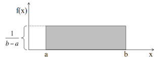
F(x) = 1/ b-a
Where ,
X uniformly distributed if the density function
a , b Parameters
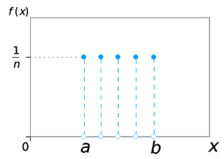
Types
This distribution has two types.
The most common type you’ll find in elementary statistics is the continuous uniform distribution and second is the discrete uniform distribution though it resembles as a rectangle but instead of a line, a series of dots are represented for the finite number of outcomes.
Example: Rolling a single die is example of a discrete uniform distribution it produces four possible outcomes: 1,2,3,4,5, or 6. There is a 1/6 probability for each number being rolled.

Uniform Distribution Example:
Let metro trains on a certain line run every half hour between mid night and six in the morning.
What will be the probability that a man entering the station at a random time during this period will have to wait at least twenty minutes.
Here, Let x denotes the waiting time (in minutes) for the next train, under the assumption that a man arrives at random at the station.
X is distributed uniformly on (0,30) with probability distributed function
f(x)= 1/30 , 0<x<30 = 0
The probability that he has to wait at least 20 minutes is
P(X.20) = 1 /30∫1.dx 20 to 30
= 1/30(30-20)
= 1/3
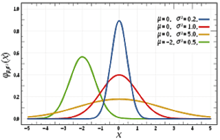
Normal Distribution
History : de Moivre developed the normal distribution as an approximation to the binomial distribution, and it was subsequently used by Laplace in 1783 to study measurement errors and by Gauss in 1809 in the analysis of astronomical data
Description: Normal distributions are common continuous probability distributions as it is highly important in statistics and are often used in natural and social studies to predict the real value random variables whose values are not known, The normal distribution, also known as the Gaussian distribution, is symmetric about the mean, differentiates data near the mean are more frequent in occurrence than data far from the mean

The Normal Equation.
Y = { 1/[ σ * sqrt(2π) ] } * e-(x – μ)2/2σ2
Where ,
X normal random variable
μ mean,
σ standard deviation
π approximately 3.14159
e approximately 2.71828.
Normal Distribution Example.
If the data is normally distributed the mean and standard deviation can be calculated ,Here if the mean is halfway between 1.2m and 1.8m
Mean = (1.2m + 1.8m) / 2 = 1.5m
95% for 4 standard deviations(2 Standard Deviations on either side)
one standarad deviation = (1.8m – 1.2m)/4
= 0.6m /4
= 0.15m
The mean and standard deviation for the normally distributed data is obtained as 1 .5m and 0.15m(one standard deviation).
Leverge your Biggest Asset Data
Inquire Now
Conclusion:
Statistical Distributions are widely used in many sectors, like Computer Science, Science, Finance, Insurance ,Engineering , Medical, Stock Market and the day to day life .
The key for good data analytics is obtained by fitting the right distribution to the data and preserving the best Estimation.
The above Distributions are observed and used in day to day life as it can be related and compared and analyzed with other distributions.