- January 4, 2019
- Posted by: Magesh Rajaram
- Category: Data & Analytics

Imagine a marketing head of a laptop manufacturer trying to wrack her head how to market her brand. Research shows that the brand is overpriced, but at the same time customers are liking the configuration compared to other brands, another insight from the dealer network says that customers are attracted to accessories than the other two. Whether she has to reduce the price or advertise the configuration better or bundle some accessories with the products. She has 3 options in mind. How can we help her?
Decision makers, when flooded with choices, choose an intuitive one, because they are the decision makers.
Check out our Advanced Analytics Services
Read More
Paucity of time, gut feel, experience are the reasons stated. If you wanted to take an analytic decision, you would throw the reasons to the bin and will commission a simple experiment.
Collect data for the individual choices, Ceteris paribus, and compare them. ANOVA is here to help, the father of statistics Fischer didn’t invent it for no reason.
ANOVA
Analysis of Variance (ANOVA) is a commonly used technique by statistical practitioners to compare two or more populations.
Specifically, the samples’ variances are compared to check if there are differences between these populations.
It had It’s origins in Ronald Fischer’s crop experiments to find the difference in the yields based on the fertilizers used.
Just like any hypothesis testing, ANOVA has the null hypothesis which states that all the means are equal.
And hence the alternative hypothesis reflects that at least for one pair of means differ.
H0: mu1 = mu2 = mu3
Ha: mu1! = mu2! = mu3
If there are j samples, then we have the means as xj bar for each sample or treatment and a grand mean x double bar.
We can calculate the difference of means between each sample and grand mean, which gives the proximity of every treatment mean to each other. This measure is called SST (sum of square for treatments)
SST = summation of j from 1 to k ( nj (xj – x double bar)2 )
As the SST increases, the variation between the treatments is high. But how high it is? To find that we incorporate another sum of squared measures known as SSE.
Just like we have variation between the treatments, there is variation within the treatments which can be defined as SSE (sum of squares for error)
SSE = summation of j from 1 to k (summation of I from 1 to nj) (xij – xj)2
= summation of j from 1 to k (nj – 1) sj2
Once we have the SSE and SST we average it for their counts of between treatments and within treatments.
MST = SST / (k-1)
MSE = SSE / (n-k)
k-1 and n-k are degrees of freedom for between and within treatments.
The final test statistic given as a respect to Fisher, and known as Fischer value is calculated as
F = MST/ MSE
To check if this F statistic is large enough to reject the null hypothesis we have to check and reject the null hypothesis if
F > F.05, k-1,n-k
Or we can go by the p-value method to find P (F > F.05, k-1,n-k) and reject the null hypothesis if the p-value is less than 0.05.
A point to be noted here is there is only factor involved which is the strategy (known as treatments), hence this method is called 1-factor ANOVA.
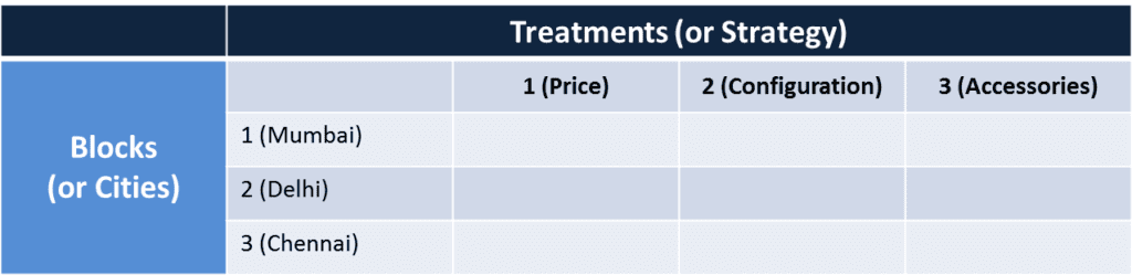
However, to add complication to this, let us say this experiment was conducted in 3 cities and hence the variation in means could be because of the strategy or city.
To rephrase it in hypothesis testing terms, it could be because of the treatments of the blocks.
Visually it can be represented as

Once we calculate the block means, treatment means and block means, the table transforms like this.

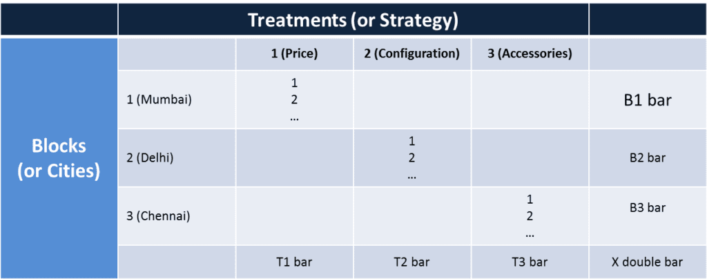
Now we have five sum of squares,
SST = r * t * summation of j from 1 to k ( nj (Tj – x double bar)2 )
SSB = r* b * summation of j from 1 to b ( nj (Bj – x double bar)2 )
SSTB = r* summation of j from 1 to k (summation of i from 1 to b) (xij – Tj – Bi + x double bar)2
SSE = summation of j from 1 to k (summation of i from 1 to b) (summation of k from 1 to r) (xijk – every cell mean)2
SSTOT = summation of j from 1 to k (summation of i from 1 to b) (summation of k from 1 to r) (xijk – grand mean)2
We average it for their counts of between treatments, between blocks and interaction between blocks and treatments.
FT = MST / MSE
FB = MSB/ MSE
FTB = SSTB / MSE
k-1, b-1, (k-1)(b-1) and n-bk are degrees of freedom for between treatments, between blocks, interaction effect and error, used in calculating the mean squares.
To check if this F statistic for treatments is large enough to reject the null hypothesis we have to check and reject the null hypothesis if
F > F.05, k-1,n-k
Or we can go by the p-value method to find P (F > F.05, k-1,n-k) and reject the null hypothesis if the p-value is less than 0.05.
Similarly, we can test the significance of variation in the blocks and interaction effects as well.
It is used in marketing and operations frequently by designing the samples carefully. Researchers split the factors and the levels and test for the significance in the variation.
It is a preliminary step in regression analysis when the regressed output is checked if the variation explained is significant or not.
Is Your Application Secure? We’re here to help. Talk to our experts Now
Inquire Now
Applications in Business
ANOVA a specific case of hypothesis testing is used widely when people encounter the problem of which factor is influencing the response variable. Some instances are
- the factor which is causing the manufacturing defect
- the effectiveness of different medicines in the healthcare industry
- the type of strategy to employ in marketing
- the features that are salient in the product development
- the marketing medium that is affecting sales