- February 28, 2017
- Posted by: Ashish Kumar
- Category: Data & Analytics

The advent of sharing economy has brought a sea change in the way urban populace commute locally.
The Ubers, Lyfts and many other local players have made taxi riding convenient, affordable and safe.
These rides have emerged as a strong alternative to the public transport clocking millions of rides per month in some cities.
The emergence of hyper-local delivery models to optimize the supply chain has also led to a large number of daily trips by these vehicles.
These developments have mandated the installations of either standalone or smartphone app-based GPS devices to keep track of and better regulate these rides and a fleet of taxis.
These GPS systems spew a ton of data generating up to GBs of data per second. With the automobile & technology experts predicting that self-driving cars would replace human-driven cars in no more than a decade, the volume and velocity of GPS data is only set to increase.
With that context in mind, it becomes imperative to understand the GPS data and the kind of insights which can be obtained by analyzing it.
A GPS or a GPS-enabled device can produce all or some of the data points mentioned below at a specified frequency (generally one record per second):
Coordinates
The latitude and longitude values are the primary data points provided by GPS devices. A set of latitude and longitude values is sufficient to locate a point on the earth. For example, (51.5007° N, 0.1246° W) denotes Big Ben in London.
Just to brush up, latitude is the angular separation of a point from the equatorial plane in north or south direction while longitude is the angular separation of a plane containing the point in east or west direction relative to the plane containing the prime meridian.
A collection of latitude and longitude values over time can reveal the trail followed by the vehicle.
Direction
This data point denotes the geographic direction in which the vehicle is moving at that instant.
A direction of 450would mean that the vehicle is headed in north-west direction while 2250 would mean that is going in south-west direction. North is taken as the reference (00)
Speed
The instantaneous rate at which the vehicle is travelling.
Timestamp
A timestamp data point can be stripped to get year, month, day, hour, minute and second information from each record
Additional data
GPS enabled devices can also send additional information like whether a taxi is carrying a passenger or not or the amount of payload a truck is carrying.
These become very powerful when combined with the coordinates and timestamp data.
Since the size of GPS data, more often than not, is huge, it makes sense to load such data into distributed file frameworks like HDFS and then process it using tools like Hive and Spark.
The processed results can be visualized in tools like R Shiny, Tableau, D3.js and Excel. If the data size is small and if one is interested in prototyping an analytics use case then Python can be used as well.
Inquire now for free consultation with our GDPR Compliant expert
Read More
With such rich data at our disposal, a variety of analytics use cases can be performed depending upon the business context. The most common of them are as follows:
1) Distance between two points
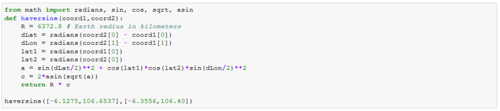
The coordinates of two points can be used to calculate the radial distance between them. Most frequently, a central point of a city is chosen as the base and the distance of the vehicle from this base is calculated at different instants of time. The distance is calculated using what is called as Haversine formula given by following expressions. Assume there are two points P1(lat1, long1) and P2(lat2, long2). The radius of the earth is R. Then
dlat = lat1 – lat2
dlong = long1 – long2
a =〖(sin(dlat/2))〗^2+cos(lat1)*cos(lat2)*〖(sin(dlong/2))〗^2
c = 2 * arcsin (√(a ))
distance = R * c
dlat and dlong should be converted to radians before calculating a.
The implementation of this calculation in Python can be done as shown below:
2) Dividing a an area into square grids
If a city or town can be divided into multiple grids of a specified equal size and insights are obtained for these individual grids, it becomes much easier to implement those insights.
Here is an abridged recipe for how this can be achieved (a detailed one would require a blog of its own):
- Decide a center for the city along with the number and the size of the grids wanted. Suppose you want 900 1km X 1km grids. You would need a square of side 30km.
- Find the line of constant longitude at a distance of 15km from the chosen center on either side (left and right) of the center. Similarly, find the line of constant latitude at a distance of 15km on top and bottom sides from the center. These lines would give the edges and their intersection would give the vertices of the overall square
- Find the latitudinal and longitudinal span of the edges and divide the span into 30 equal parts. Call them latd and longd. Start from one edge to reach the other edge by incrementally increasing the latitude and longitude by these values.
- Draw lines of constant longitude and latitude at those points. This would result in 30 vertical and 30 horizontal lines and their intersection would produce 900 grids with all their vertices with known latitude and longitude
These grids can be visualized using leaflet library in D3.js or R Shiny.
3) Temporal averages of important metrics
The timestamp data can be used to gauge trends about the additional data across various timeframes. For example, daily averages of distances covered in each hour.
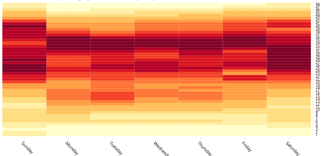
These time frames can be nested as well to get a more granular picture e.g. a plot of average payload for each half hour of the day for each day of the week.
The relevant time element needs to be gleaned out of timestamp followed by a grouping of the relevant metric column by the time element. An indicative temporal visualization would look as the one shown below.
The horizontal axis shows the day of the week while the vertical axis shows the half hour of the day while the metric has been shown as the heat map gradient.
Geospatial analytics can unravel many mysteries and can help organizations optimize taxi routing to match supply and demand, fight pilferage and related frauds and minimize the chances of accidents or the damage caused by it.