Loan Defaulters Prediction

Loans are instruments for a bank to generate revenue from it’s capital derived from fixed deposits.

It is a differential interest business when we compare the lending rate of the bank to the customer and the borrowing rate of the bank from the Federal Reserve.

In the case of tightrope business, it becomes cardinal to tighten any leakages of revenue via delay in interest payment and capital erosion by default.

Just like any other industry, where the payment is to be performed after the product purchase, there are bound to be defaulters and late payees. In financial services, it is cardinal to track every customer based on his behaviour.

Besides the initial checks for his loan paying ability by checking the credibility score and demographical variables, there is a behaviour pattern that gives rich insights on the customer’s payment behaviour.

And when the transaction behaviour is combined with demographics and the product characteristics which in this case can be the interest rates, loan period, installment amount and others, it throws up light on what the customer is bound to do – whether he is going to delay, pay on time.

This type of modelling is called Propensity Modelling. It is used in a variety of cases such as propensity to buy, default, churn.

The Defaulters’ case

A financial services company was already monitoring the customers by a factor – that is if he has delayed his payment.

Once a customer delays he gets into the blacklist, on the other hand, the customers who are prompt are always in the whitelist.

Is there more to this logic we can build? We have important variables on hand – the mode of payment, the days between payment and the due date.

Then there are loan characteristics like interest rate, time period, installment amount and others.

Using these, we can build a statistical model to tighten the logic. The objective of the model is prediction of the default. To refine it further can we classify the customers as defaulters and non-defaulters.

While the classification of customers as defaulters and non-defaulters sound more clear and exciting, in the models we don’t get labels but a numeric score, in this case, a probability of default based on the combination of characteristics.

We can utilize this probability to define a threshold for defaulters or non-defaulters. Often the business comes up with these definitions of the customers, in this case, it was decided to have three types – Least Risky, Slightly risky, Risky, just like a modified 3 rating Likert Scale.

There are many classification models in use – decision trees, logistic regression, XG Boost models, and Neural Networks.

Exploratory Analysis

Before touching the modelling tasks, it is fundamental to understand the data and fix up issues.

A preliminary exploratory data analysis (EDA) on the distribution of variables, find the missing values, correlation between the variables. It gives answers to these questions.

• How to do missing value imputations?
• Are there variables we can dismiss by empirical methods?
• Can we get some important insights from EDA?

Correlation

For example, when performing correlation test some variable combinations such as gross loan- net loan, balance amount- Loan status might show a high correlation.

One of these variables has to be removed to increase the explaining ability of the model. Also, it decreases the computation complexity with fewer variables.

Box Plots

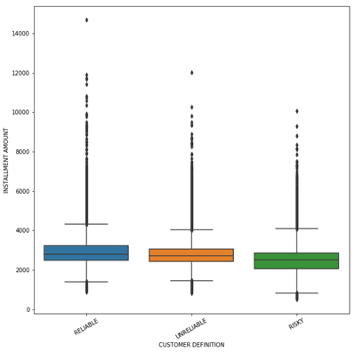
Some plots that will help us know about the distribution of variables are box plots. They give the distribution of the variables.

For instance, when the installment amount was plotted for 3 types of customers (Least risky to Slightly to Highly Risky), the distribution of highly risky was lower than the least risky customers.

De-facto, our assumption might have been as the installment amount increases the risk increases, whereas this plot threw that assumption upside down.

With the increase in installment amount, customers were paying better. A plausible explanation could be the customers are lethargic when the amount is low. Possibly!

Bar Plots

Cross-tabulations of some important variables gives a relationship between the variables. At the bare minimum, the risk category and variables like tenure, installment amount shows up good insights.

To quote the case of tenure tabulated with the risk type, as the tenure increases the risk of default increases.

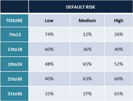
A reasonable explanation could be, customers become lethargic when the commitment period is long, so much common for the business and life!

Looking into other variables like the vehicle make in case of auto loans, the house type purchased in case of home loans can give important insights.

Certain vehicle makes or house types can be more prone to default, the significance of the relationships can be tested using Chi-square tests.

Modelling

An XG Boost model was fit on the data to find the probability of risk of default.

The training to test ratio can be set at a standard size of more than 60: 40. To give more allowance for training and at the same time not ignoring the size of the testing set, we kept the ratio at 70:30.

A variable importance test is one which ranks the variables that explains the explanation power of independent variables to dependent variables.

A random forest model was run to find the ranks of variables. Some important loan characteristics like interest rate, installment amount, loan amount were the usual suspects.

XG Boost algorithm develops on the decision tree model by voting the best classifying decision trees.

The subsequent model trained develops on the errors of the previous model, hence it has a starting point from the previous model.

We fine-tuned parameters for the model to improve the accuracy. For example, the number of trees, as there were less than a million records we fixed this as 40.

The max depth was kept at 8 as we have reduced the number of significant variables to be input in the model to 15. The learning rate was experimented with values of 0.1 and on both sides.

The confusion matrix was generated to find the accuracy, prediction and recall.

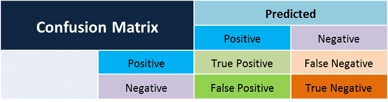
Just to explain the accuracy, it is how accurately the model predicts the positives and negatives.

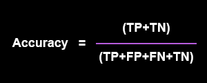
The accuracy turned to be consistent at about 70% when cross-validation was done by random cutting to generate 10 runs of the model.

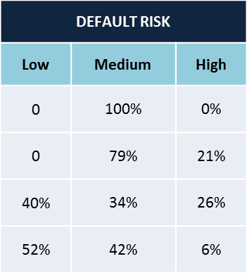
The classification model was scored on the real-time customer database. It shows up three probabilities for every customer, one each for Least risky, slightly risky and highly risky. For some customers,

• Case a – it can be a clear demarcation with one of the probability tending to 1
• Case b – for others the probabilities can be evenly split.

LIME outputting

LIME is the abbreviation for Local Interpretable Model Agnostic explanations. Many of the times, business requires simple explanations in short time, they don’t have time to wrap their head around the measures like variance, significance, entropy etc.

and how they combine to explain the classification of labels. When a customer is presented to be with high risk for default, how can we explain that to business in simple terms?

LIME does that for us, it explains how each variable is powering the classification. Although it cannot be precise, it is an approximate explanation of why the model is tending to classify the customer as such.

The image below shows an example of different variables at interplay to predict the customer’s risk type.

Putting everything together to use

We have a set of insights coming from the EDA, the model is throwing up the risk metric and the LIME outputs are interpreting the model results. How to get the acts together with the three components?

The main advantage of doing an EDA is it gives heads up insights. At a very early stage, the business can post red flags for certain customer types.

As seen earlier, we will be able to predict a defaulter, even before the person defaults once by taking into consideration the variables combinations like instalment amount, period of the loan, interest rate.

The set of insights are automated and can be run every quarter or six months to generate the red flags.

The Classification model being the main component, predicts the default risk. The probability of the customer to default can be used in many ways by business.

• The operations team can take up the top decile of the risky customers, monitor them closely and frequently.
• The sales team’s incentives can be tuned as per the default risk.
• The marketing team can focus on campaigning for targeting certain vehicle makes or house types, certain geographies as they know which are more prone to default.

To judge fairly a machine output, we have to give allowances to some really tricky and wacky predictions from machine learning.

It completely runs by past data and hence some predictions can be completely wrong. 

LIME function helps in digging deep into those cases and understand the logic and rules employed by the model.

It will be able to give the exact reason as to why a person is classified as such, maybe a new line of thinking to the business.